Solving the
Time-Dependent-Schroedinger Equation

Evolution of a particle in different potentials:
free, step, square, harmonic

This research project was part of my MSc Physics at Imperial College London in 2021 - one week project.

As part of my studies at Imerpial I embarked on a 1 week project. I did chose to play around with the centrepiece of quantum mechnaics - the Time-Dependent Schroedinger Equation (TDSE):

$${i \hbar \frac{\partial}{\partial t} \Psi(\mathbf{r},t) = H \Psi(\mathbf{r},t)}$$

Motivation

The aim of the 1 week project built something cool with Mathematica. Having dealt with the time-independent version of the Schroedinger Equation in countless probelem sheets and exams, problems and exercises with the time-dependent version always seemed very distant. I wanted to gain intition via a nice animation.

This was the goal: Gain Intition of the TDSE in the standard potential wells.

Project Summary

In this project the time-dependent Schrödinger Equation has been solved using the 'Finite Domain Time Difference Method' for different simple static potential wells for a Gaussian wave packet.

The behaviour of the particle waves exhibits the inherently quantum mechanical behaviour that is expected. The animations generated allow to gain physical intuition.

Theory

The equation to solve is the time-dependent Schrödinger Equation (TDSE):

$$ i \hbar \frac{\partial \Psi(x,t)}{\partial t} = H(x) \Psi(x,t) $$

with H(x) the static Hamiltonian. For simplicity here a static potential was chooses.

$$ H(x) = -\frac{\hbar^2}{2m} \frac{\partial^2}{\partial x^2} + V(x) $$

The TDSE can be rewritten applying the standard "Finite Time Difference Method" (see here):

$$ \frac{\partial \Psi(x,t)}{\partial t} = \frac{\Psi(x, t + \Delta t) - \Psi(x,t)}{\Delta t} $$ $$ \frac{\partial^2 \Psi(x,t)}{\partial x^2} = \frac{\Psi(x, t + \Delta t) - 2 \Psi(x,t) + \Psi(x-\Delta x,t)}{\Delta x^2} $$ Substituting this into the TDSE yields: $$ \Psi(x, t+\Delta t) = \Psi(x,t) - \frac{\Delta t \hbar}{2 i (\Delta x)^2 m} \Bigg[ \Psi(x+\Delta x,t) -2 \Psi(x,t) + \Psi(x-\Delta x, t)\Bigg] + \frac{\Delta t}{i \hbar} V(x) \Psi(x,t) $$ where we define the constants as $$ c_1 = \frac{\Delta t}{2 (\Delta x)^2 m} $$ and $$ c_1 =\frac{\Delta t}{\hbar} $$ Then taking the real and imaginary parts of the wavefucntion one finally arrives at the equations used for the calculation: $$ \boxed{ \Phi_R(x,t+\Delta t) = \Phi_R(x,t) - c_1 \Bigg[\Phi_I(x+\Delta x, t)+ 2 \Phi_I(x,t) +\Phi_I(x-\Delta x, t) \Bigg] +c_2 V(x) \Phi_I(x,t)} $$ $$ \boxed{ \Phi_I(x,t+\Delta t) = \Phi_I(x,t) + c_1 \Bigg[\Phi_R(x+\Delta x, t)+ 2 \Phi_R(x,t) +\Phi_R(x-\Delta x, t) \Bigg] +c_2 V(x) \Phi_R(x,t)} $$

These two equations are the core of the simulation. For the purpose of generating a meaningful animation the constants c₁ and c₂ have been slightly adapted.^[1]

The wavefunction defining the particle to simulate is chosen to be an well defined electron. In order to define the particle well a Gaussian wave packet is chosen. For a Gaussian wavepacket a single wavevector can be defined as its Fourier transform frequencies are clustered around that single wave vector. This allows to define a somewhat localized particle. The Gaussian wavepacket is: $$ \Psi(x, 0) = \Phi_0(x) = \frac{1}{\sqrt{\sigma \sqrt{\pi}}} e^{- \frac{x^2}{2*\sigma^2}} $$ let us define the normalisation as: $$\sqrt{\sigma \sqrt{\pi}} = A$$ Then the modulated real and imaginary parts are \begin{equation} \Phi_R(x,0) = \frac{1}{A} e^{-\frac{1}{2} \big( \frac{x-x_0}{s} \big)^2} cos[k (x-x_0)] \end{equation} \begin{equation} \Phi_I(x,0) = \frac{1}{A} e^{-\frac{1}{2} \big( \frac{x-x_0}{s} \big)^2} sin[k (x-x_0)] \end{equation} where the normalization constant can be found by integration according to the Born Rule: \begin{equation} 1 = \int_{-\infty}^{\infty} |\Psi(x,t)|^2 \,dx \end{equation} The particles momentum is specified using the deBroglie relations: \begin{equation} p = \hbar k \end{equation} where k is the wavevector defines as: \begin{equation} k = \frac{2 \pi}{\lambda} \end{equation} The potentials chosen to present here are all finite potentials:

• finite square well
• finite step well
• quadratic/harmonic

The default particle presented has a wavelength $$\lambda = 30 nm$$ and a rest mass m = m_e. Therefore the energy of the chosen electron particle has a kinetic energy as a free particle given by the deBroglie relation as: \begin{equation} E = \hbar \omega = \frac{h c}{\lambda} \approx 6.625*10^{-18} J\approx 41.35 eV \end{equation} Therefore to explore the interesting behaviour of a bound particle we choose the welldepth or wellheight to be 80eV.

Aims & Objectives

Aims

• solve the time dependent Schrödinger equation using the 'Finite Domain Time Difference Method'
• demonstrate the working method on a few potentials
• comment on physical intuition gained

Objectives

• discretize space and time
• implement a physical potential parameters
• implement physical particle/wave parameters
• generate potential wells: free, square, harmonic, step
• demonstrate potential wells

Results

See Sum-up video here: The individual simulations are also shown here:

Finite Square Well

Finite Square Well

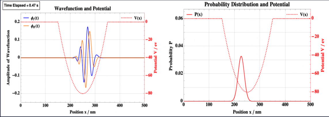
Quadratic Well

Step Well

Note the obvious quantum tunneling here.